1.1 Scatter and Line plots

The most commonly used plot type is the scatter plot or line plot. For this example, we’ll make a plot of the sine function in the interval \(0,2\pi\)

x <- seq(0, 2 * pi, length.out = 50)
y <- sin(x)

plot(x = x, y = y)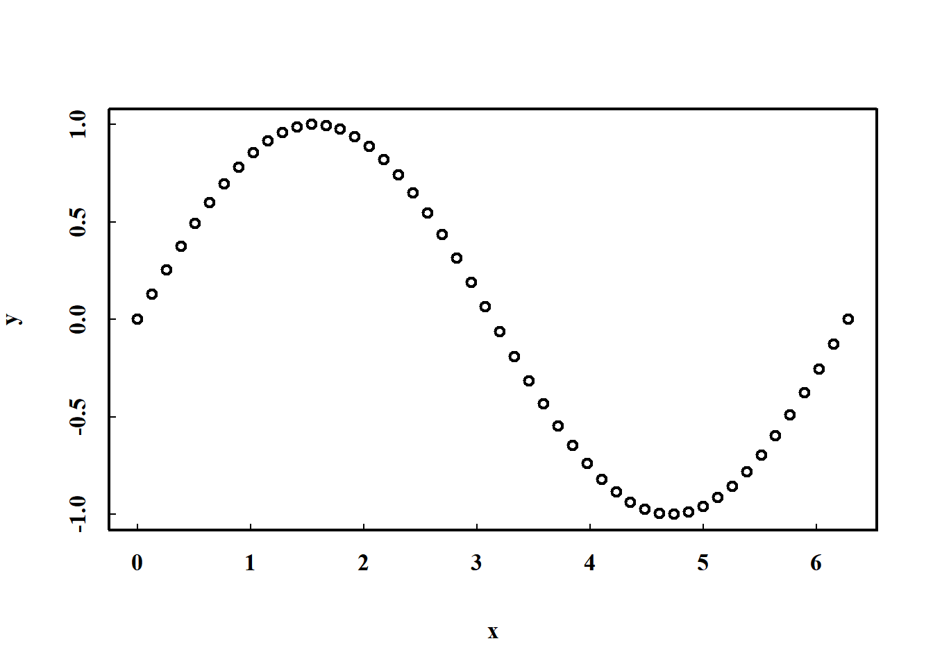

It’s important to note that when a call to the plot(x, y,...) function is made, the following events occur:

• A new plot device is created

• A new plot window is activated within the plot device

• The values defined in the vector x are stored as the \(x\) coordinates of the points \((x_i,y_i), i=1,...,n\)

• The values defined in the vector y are stored as the \(y\) coordinates of the points \((x_i,y_i), i=1,...,n\)

• If x and y contain the same number of elements, the points \((x_i,y_i), i=1,...,n\) are printed in the active plot window

Additional arguments, denoted by ... are then executed to change the active plot device settings as shown below. If values for these arguments aren’t specified, R will use default values based on the type of objects being plotted.

x <- seq(0, 2 * pi, length.out = 50)
y <- sin(x)
plot(x = x, 
     y = y,
     xlim = c(0, 2*pi),
     ylim = c(-1, 1),
     type = 'p', 
     main = 'Title',
     sub = 'Subtitle',
     xlab = 'x-axis label',
     ylab = 'y-axis label',
     xaxt = 's',            # show 's' or not-show 'n' x-axis
     yaxt = 's',            # show 's' or not-show 'n' y-axis
     axes = TRUE,           # show axes?
     ann = TRUE,            # show plot annotations?
     pch = 1,               # Sets the type of plot character
     col = 1,               # Change the color of plotted objects
     cex = 1,               # Enlarge size of plotted objects
     cex.axis = 1,          # Enlarge axis values
     cex.lab = 1,           # Enlarge axis labels
     cex.main = 1.3,        # Enlarge plot title
     col.axis = 1,          # Color axis values
     col.lab = 'red',       # Color axis labels
     col.main = '#d3d3d3',  # Color plot title
     las = 0)               # Rotate axis values 0,1,2,3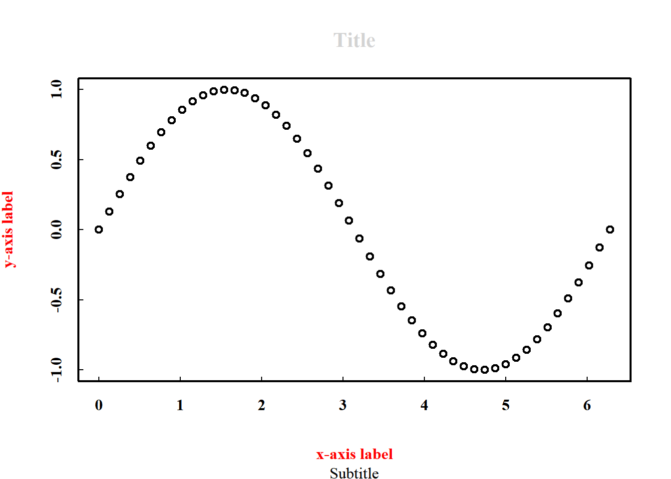

1.1.1 Changing plot type

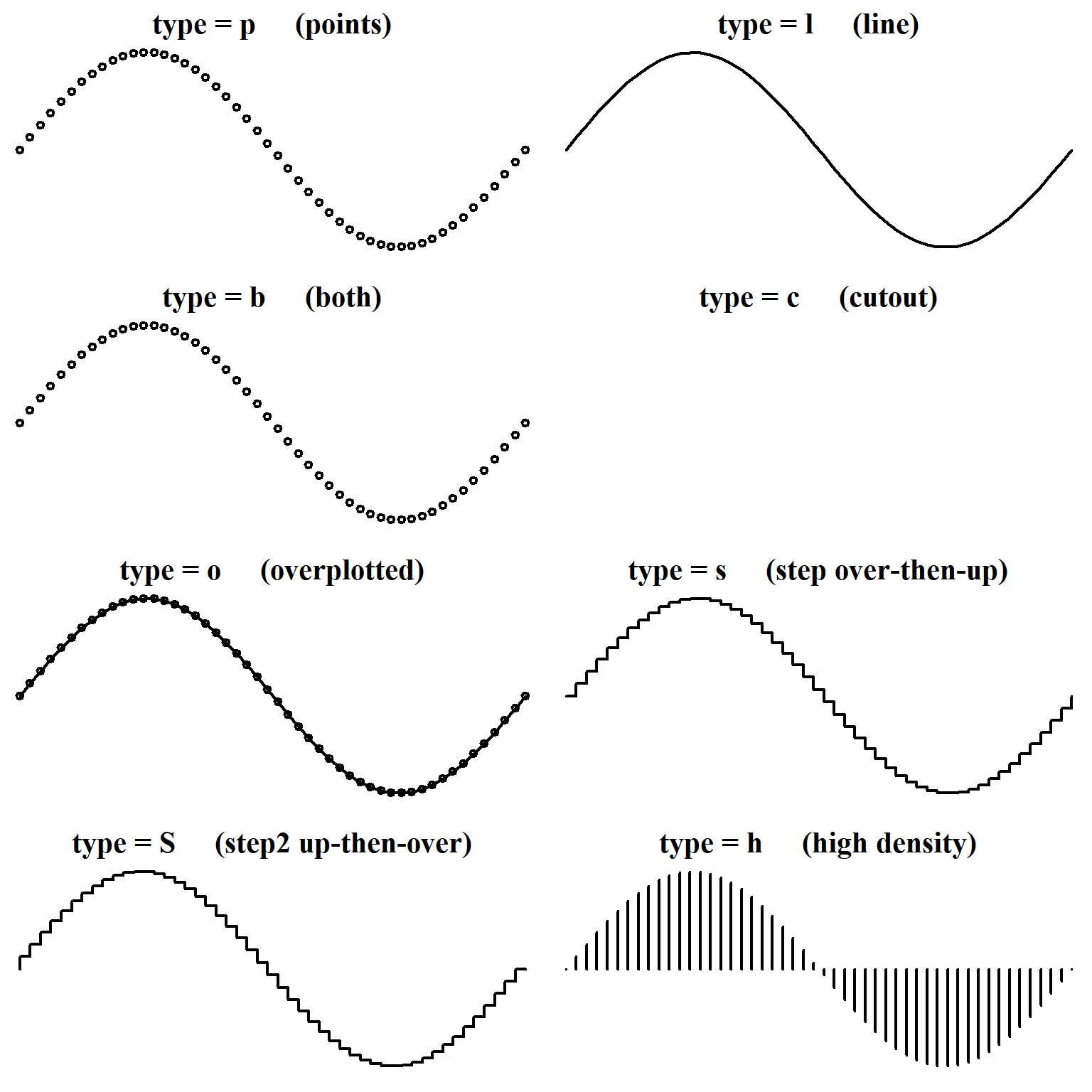
By default type = 'p', meaning that the values provided for x and y will be plotted as points. However, eight different plot types may be created simply by changing the type argument.

1.1.2 Custom plot characters

For plots in which type = 'p' the plotting character pch and color col can be specified numerically. Figure . shows the 256 distinct plot characters and colors that can be defined numerically.

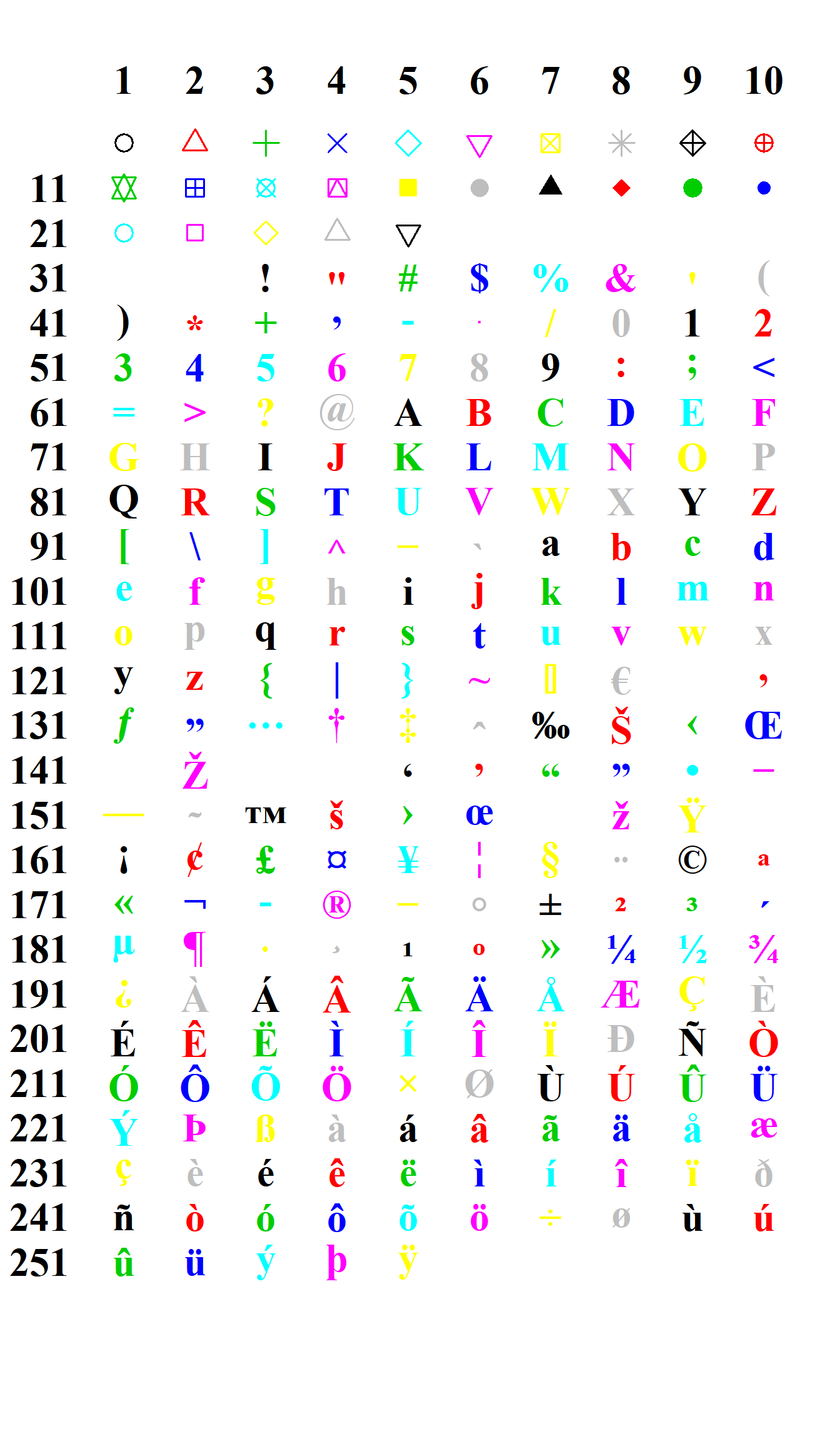
Figure .: Available plotting characters for base R graphics

These arguments may also be specified explicitly, for example pch = '?' and col = 'red'

x <- seq(0, 2 * pi, length.out = 50)
y <- sin(x)

plot(x = x, 
     y = y,
     pch = '?',
     col = 'red')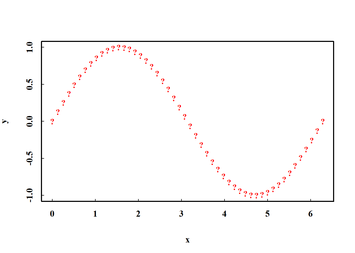

The size and color of each plot character can also be customized

x <- seq(0, 2 * pi, length.out = 50)
y <- sin(x)

plot(x = x,
     y = y,
     pch = 16,
     cex = c(seq(0.5,12.5,0.5),seq(12.5,0.5,-0.5)),
     col = rainbow(50),
     las = 1,
     cex.axis = 1.25)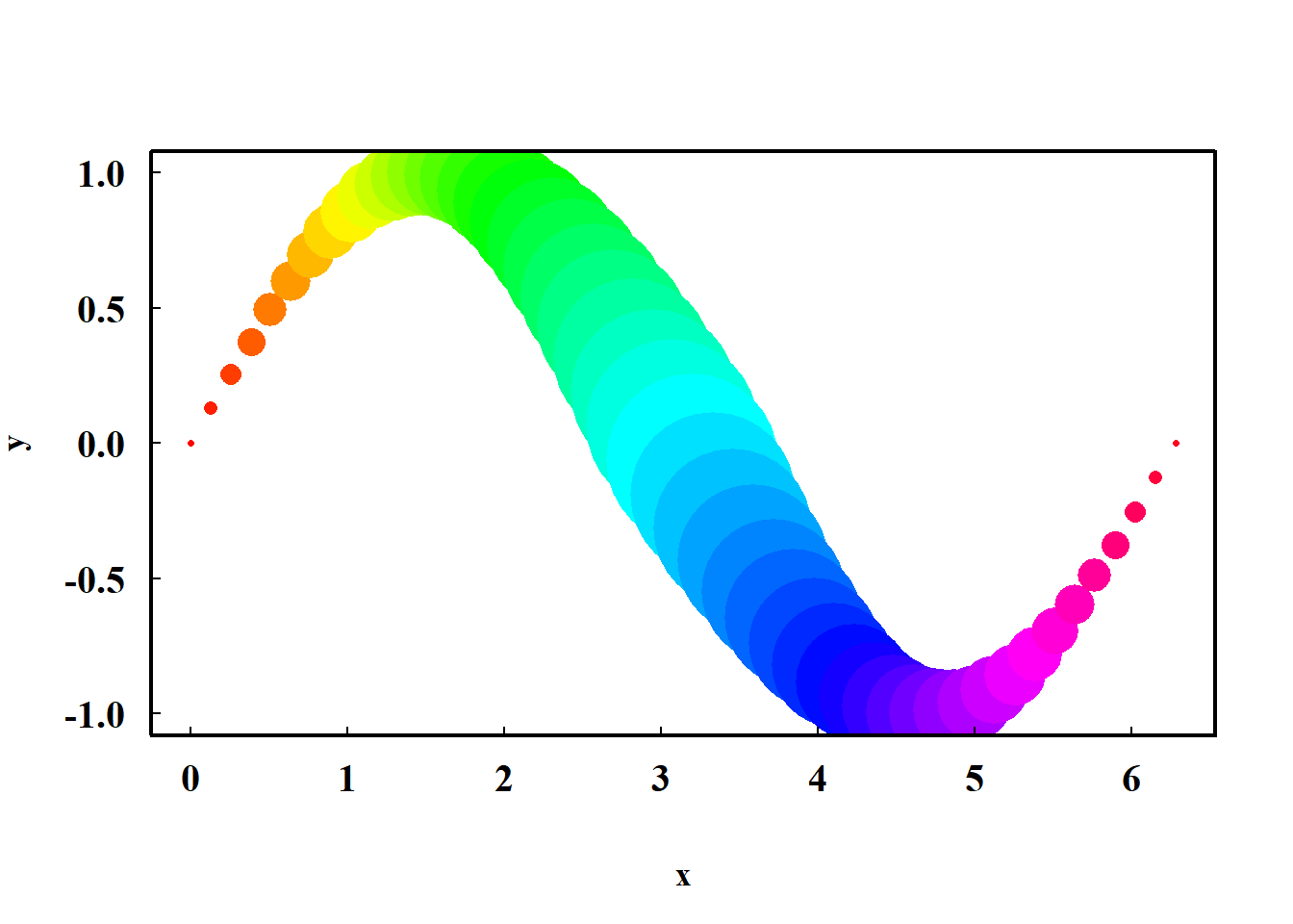

1.1.3 Custom lines

When type = 'l' the points are connected by lines. The line type and line width can be customized using the lty and lwd arguments, as shown in Figure . below.

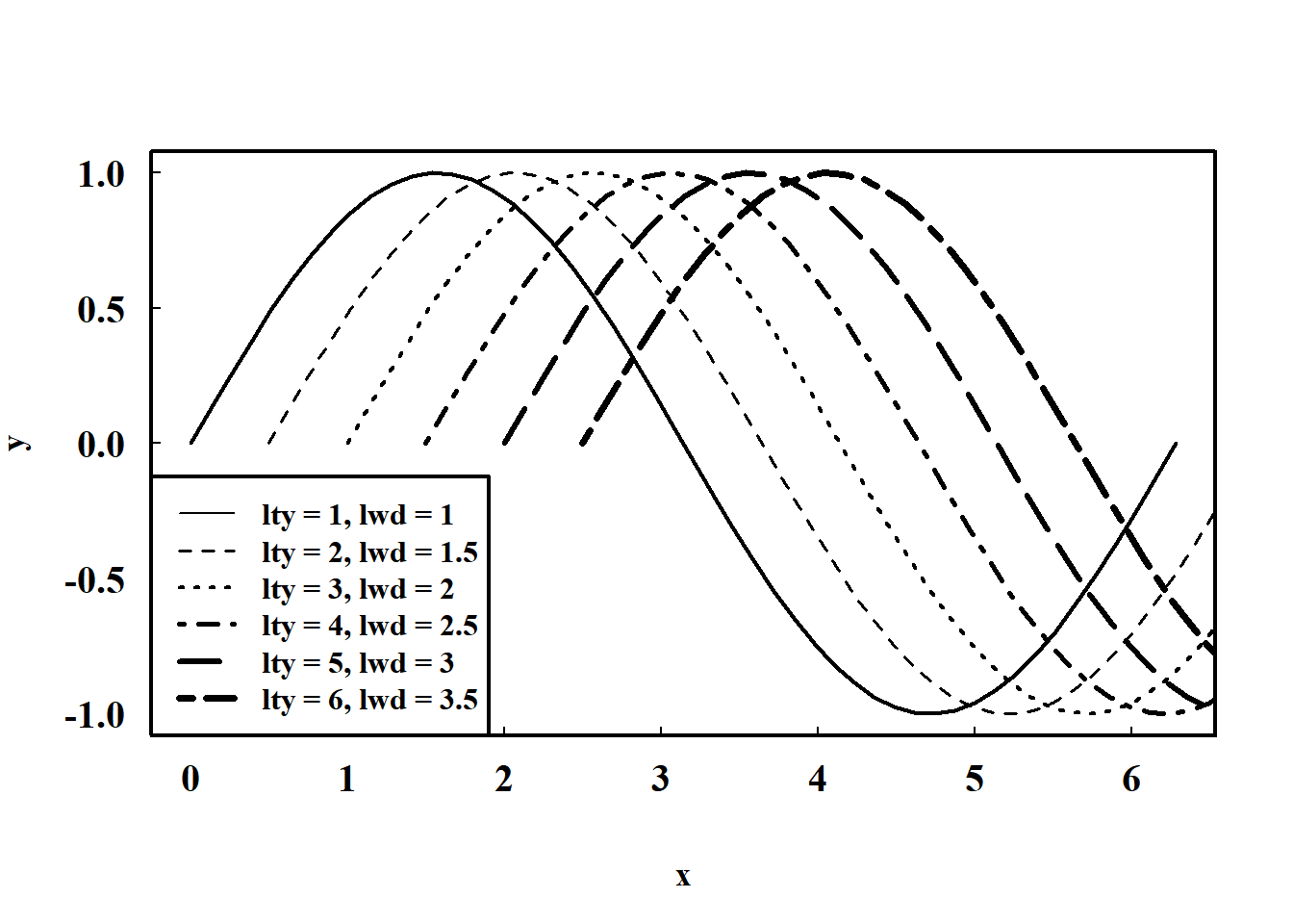
Figure .: Examples of custom line types and line widths in R base graphics